
Matthew Leitch, educator, consultant, researcher
Real Economics and sustainability
Psychology and science generally
OTHER MATERIALWorking In Uncertainty
Risk modeling alternatives for risk registers
First published 5 June 2003.
Introduction to the design problem
This page is for people who want to design a useful and efficient way to quantify risks on a risk register. Perhaps you already have a process that generates a risk register each period with some kind of risk ratings but you want a better way. Perhaps the existing method is illogical.
When designing a risk management or modeling approach it is easy to end up with something that is completely inappropriate. Risk management has developed separately in different disciplines for different uses. Often, the methods and concepts of risk used in one discipline are fundamentally different from those in another. Problems arise when ideas taken from one style of risk management and its normal area of application are applied elsewhere.
Coming up with something logical and practical is hard. Partly this is because quantifying risks is hard. Often there is little data to back up gut feeling. A risk may be something for which there is no relevant history. Gut feeling is notoriously unreliable. Other problems include the fact that risks combine in ways that are difficult to think about and quantify. There is a risk of getting the structure of the model itself wrong, a problem whose impact is difficult to quantify.
Despite this, amazing things can be done by very intelligent people, backed by extensive empirical data and computers, to quantify and visualise risks, often discovering things intuition did not bring to light.
Unfortunately, in other settings this sophistication is not available or hard to justify. Many risk ratings are done by asking groups of people to make subjective ratings and many of these are fundamentally flawed. The most common mistake is to make independent ratings of ‘likelihood of occurrence’ and ‘impact on occurrence’ for ‘risks’ that are really sets of outcomes having varied impacts. (An example is ‘risk of loss of market share"; doesn't the impact depend on how much share is lost?) This is common in Turnbull compliant risk rating in UK listed companies (done as part of the internal control system), for example.
This web page looks at alternative approaches to risk rating and where they are appropriate, emphasising efficiency and valid alternatives to the likelihood x impact mistake.
Typical risk register items
Another way to see the problems of designing a risk quantification scheme is to look at the sort of items that commonly appear on risk registers. Some risk registers break down risk using a consistent scheme and terminology. In others the risks are suggested in brain storming workshops and reflect different concepts of risk. Here are some typical items with comments to bring out the ideas behind each.
Example |
Comments |
|---|---|
‘Market risk.’ |
This is typically something calculated from readily available market data. Its definition may be laid down by law or regulation. Depending on the rules applied it may be that only the likelihood of extremely bad outcomes is of interest or that it is the spread of outcomes that is considered important. |
| ‘Regulation risk.’ | This just refers to all the things that might happen in the organisation's regulatory environment and their impact. Unlike ‘Market risk’ this is unlikely to be quantified, due to lack of relevant data. |
‘Collision involving passenger ferry.’ |
This sort of item often appears on risk analyses done for safety management or insurance purposes. It is a mishap that might occur and its impact is usually the cost of getting back to what you had before. Like the other risks in such a scheme this is a disembodied thing often imagined to be independent of other risks. The combined impact of these risks is often thought of as simply the sum of the individual risk impacts. |
‘Loss of market share.’ |
In contrast to the previous risk this one is not independent of other risks. Loss of market share will correlate with other risks like ‘Failure to achieve earnings target". The impact of ‘Loss of market share’ is much more difficult to estimate because many other factors also drive the financial results, which are where the impact is usually measured. This risk is a continuous one, with many degrees of loss of market share possible. |
‘Failure to harness innovation’ |
The risk of failing to do something contrasts with risks that are more to do with external conditions, or fears about financial or other results. |
‘Market demand’ |
Like ‘Loss of market share’ this is continuous and far from independent of other things of interest. What is different is that it refers to all market demand possibilities, not just the downside. |
‘Incomplete billing’ |
This is a typically ambiguous item that could refer to the risk of billing in a year being incomplete (more like a certainty for many companies) or the risk of an individual bill being missing or incomplete. This risk is at the level of a process and refers to something that (when billing is on a large scale) happens very frequently. |
Design considerations
There are some key design choices. Perhaps the most helpful to consider first are the purpose(s) of the risk assessments, the underlying theory and ultimate yardstick of risk, whether the approach should be formal and centralised or informal and decentralised or both, whether upside risks are to be considered, and whether the modeling needs to be integrated. Various other factors come into deciding the methods of risk distribution characterisation and what backs them up. Finally, there are choices about how risks are identified in the first place.
Perhaps surprisingly the type of risks included (e.g. compliance, financial reporting, safety) is not directly a consideration though each tends to have its own characteristics which drive the design. For example, equity market risks usually involve looking at the upside too, and using an integrated model (because share returns correlate to some extent), and can usually benefit from a huge amount of readily available quantitive data.
The remaining sections of this page look at these design choices.
What is it for?
The ultimate purpose(s) of the analysis is important to its design. In some cases the risk assessment is only one factor and perhaps less important than you might think:
Purpose |
Design notes |
|---|---|
To make uncertainty explicit and get people to consider it in strategic thinking, business planning, and decisions. |
This can usually be done with very little need for precision provided we accept that the future is more uncertain than we usually think and consider upside risk as well as downside. For example, instead of forecasting sales next year as �1,234,000 exactly, provide a distribution showing the probability density of various levels of sales for next year. If you don't know what the distribution should be a generously wide spread plucked out of the air is more useful and realistic than picking a single number and acting as if this is what is going to happen. If the decision is a large one, such as approval of a capital investment, more accurate quantification is usually desirable. Analyses are typically of integrated systems and encompass upside risks as well as downside. (See later for an explanation of these ideas.) Some modeling is done before objectives are set, or when objectives are unclear or changing. It needs to give attention to external conditions. |
| To know our top 10 risks. | Achieving this is surprisingly difficult. How do you keep risk sets at a comparable level of aggregation? (e.g. ‘Health and safety’ beats ‘Accidents at coffee machines’ because it is wider.) Is the risk rating before or after mitigation? And is that current mitigation or planned mitigation? Focusing on top risks may be helpful but not if those risks are already well covered or cannot be covered, as no actions arise. You could be overlooking worthwhile mitigation of other risks. Another approach is to divide your total set of risks into 10 categories, each of roughly equal importance. This is more informative for something like an Operating and Financial Review or other public discussion of key risks. |
To categorise items in a population (e.g. chemicals, companies, customers) according to their riskiness so that different policies can be applied to members of each category. |
Ideally the categorisation will show an estimate of the probability and/or impact of the risks in question but this is not essential. Many such ratings are just indexes. |
To prioritise risk management work and/or expenditure. |
High risk is one reason to spend time thinking about possible management actions. However, risk is only one factor. Others include the scope for successful action, the likely cost of action, and past lack of attention to an area. The complexity of the issues is also an indicator of how much thinking is likely to be needed. Finally, risk management actions take time to put in place so prioritising risk management work usually involves anticipating the need for management actions and starting work in the right areas in good time. |
To consider the impact of a proposed risk management action, perhaps choosing one from alternatives. |
This is usually done by quantification of the risk with and without the proposed risk management action. Ideally, risk management actions will form an integrated system and so ideally it is combinations of actions that need to be evaluated. This makes the analysis much more difficult. Typically, the system would be designed by using rules of thumb (also known as design heuristics) with very few, if any, quantified evaluations. |
To calculate regulatory or capital requirements, or estimate the chance of financial failure. |
Regulatory and economic capital are related to the chance of financial failure in a given time period. The smaller you want the chance of failure to be the more capital you need to start with. Regulatory capital tends to be less than you really need (i.e. economic capital) because regulations usually do not take into account all types of risk. The modeling involves all required risks, upside and downside, and gets quite technical. Working out the risks of the most extreme outcomes is particularly difficult to do accurately since there is so little experience of these conditions, and even getting them to happen often enough in simulations can take a lot of trials. |
To try to ensure that objectives will be achieved. |
This tends to be the approach applied in corporate governance and is preferred by accountants and auditors. It normally involves identifying objectives and then reasons why they might not be achieved, then trying to think of ways to mitigate those risks. In this approach upside risks are not considered because the thinking assumes that nothing is better than achieving your original objectives. |
The conclusion from the above lists is that knowing how much risk you face is not always very helpful and often needs to be supplemented by considering other factors. The best option may be to rethink the risk register more fundamentally, bring in other factors relevant to the decisions being made, and perhaps make risk quantification even simpler and cheaper than before. For an example of this see ‘A new focus for Turnbull compliance.’
Risk quantification is perhaps most important for deciding capital requirements and judging the returns from risk management actions (especially where life is at stake, such as when considering the health risks of new medicines).
The ultimate yardstick
The variety of theories of risk is astonishing. The meaning of ‘risk’ is itself highly controversial among risk experts but you don't have to be an expert to realise, for example, that there is something fundamentally different between ‘a risk’ and ‘some risk". There is little agreement and this is one of the main reasons for the variety of risk measurement and management methods.
Here are four alternative ideas about measuring risk:
Risk Measures: The most common approach in the theory of finance is to calculate expected returns (i.e. what is expected on average) and calculate another number which represents the amount of risk involved. Early theories used the variance of returns from an investment as the measure of its risk. There are now alternatives to this including formulae that do not involve squaring the difference between points on the distribution and its mean, and formulae that give a different weight to variations below the mean compared to variations above the mean. In the CAPM theory it is only systematic risk (i.e. risk that cannot be removed by diversification) that is considered.
Value at Risk: In this approach the only outcomes given any weight are those that lead to collapse of the firm or some other disastrous outcome. Given a level of confidence, the calculation sets out to estimate the amount of capital backing you would need to be that confident of avoiding collapse. Other outcomes do not get the same attention so, in effect, most of the attention goes onto circumstances that are extremely unlikely.
An indicator but not a measure: In some risk management approaches there is no measurement at all. There may just be relative ratings, points, or categorisations (e.g. ‘High, Medium, Low’, ‘Red, Amber, Green’). If the objective is to direct remedial action to the right places it may be that just knowing the most risky areas is enough.
Expected Utility: In this theory there is no separate measure of risk. The expected return is measured in utility instead of money. The theory is that it is possible to assign numbers to outcomes so that they sum up a rational person's preference for those outcomes and decisions can be made purely on the basis of maximising expected utility. (See below for an explanation.) Although there is plenty of evidence that we do not always act in accordance with this theory we would probably do better in life if we did.
Of these methods Expected Utility is particularly interesting and perhaps under-used compared to its potential. It is a practical, everyday alternative to the risk measure approach that is common in finance.
In finance and business management theory it is now common to take shareholder value as the ultimate basis for decisions. This is seen as the same as the market value of a company's shares and as the net present value (NPV) of future cash flows. Though there are variations the typical accountant's way of evaluating decisions is to try to build a model that predicts cash flows and then discount these to find the NPV of each alternative in the decision.
However, this approach struggles in the face of future uncertainty and is difficult to apply in many everyday decisions. The further into the future you look the harder it is to pin down specific cash flows. Businesses are complex systems with many feedback loops. What is the value of a satisfied customer, improved brand image, or hiring someone who has good ideas? Real decision making relies on what people like to call ‘strategic’ considerations. In other words, things we think are important but which we can't seem to reduce to cash flows.
We usually express what we are trying to do using objectives, which rarely have a quantified link to cash flows. Our objectives are things like ‘Improved customer service", ‘Higher awareness of our new services among our customers’, and ‘A more motivated workforce’. The value of different levels of achievement on these objectives is something we typically have only a gut feel for. It would be nice to be more scientific but gut feel is usually all we have time for, particularly as our plans and objectives often shift.
Expected Utility is a tool for rational decision making under uncertainty even in these tough conditions. Each objective is turned into an attribute in a simple utility formula, and levels of achievement on each attribute are described to create scales. Once you have established the attributes you value at all, and set out a scale for each, it can take just a few minutes to get a rough idea of how much you value each level of achievement against each attribute/objective. This can be done using very simple software on a web page, based on techniques called conjoint analysis.
Next, modeling tools like @RISK, Crystal Ball, and XLsim can extend ordinary spreadsheet models by adding in explicit consideration of uncertainty and translating achievements into utility terms at the end of the model. If alternative actions and their risks are modeled to estimate the effect on probability distributions of the attributes then these effects can easily be turned into overall expected utility changes.
Formal and centralised or informal and decentralised?
Most risk modeling and management approaches in use today are formal, centralised, and under the continuous control of a specialist team. However, it doesn't have to be that way. Risk management can be decentralised and under less strict control as an alternative or to complement a formal, centralised approach.
Strategic decisions by senior management about risk and uncertainty are important, but so too are the thousands of less important decisions made by managers at all levels daily. Influencing the skill with which everyone handles risk and uncertainty requires a different, more enthusing, more accessible approach.
Upside risks too?
By upside risks I mean outcomes better than some benchmark level taken as zero. That benchmark will be the planned outcome, expected outcome, or some other outcome considered ‘proper’ for some reason. For example, for credit risk the benchmark is usually that the customer pays back the loan and agreed interest on time. For investment returns the benchmark is typically the expected return. In project risk assessments the planned outcome is usually the benchmark. In many situations we have a choice.
A common view is that risk is purely to do with bad things that might happen. This makes perfect sense if you are managing safety risks, or insurable risks, to name two very important fields of risk management. However, the same approach has unhelpful implications when applied to project and general business risks. In effect it says there can be no better outcome than our plan or forecast.
Often, risk sets suggested in workshops include only part of the story – usually the downside. However, it is easy to guess the rest in most cases. For example, the rest of the risk set ‘Trouble at the mill’ is ‘No trouble at the mill’, and the rest of ‘Loss of market share’ is ‘Gain of market share or market share held.’
These are complete risk sets in the sense that the probabilities of the outcomes in each sum to 1.
If upside risks are considered as well as downside it is even more important to be clear about what the benchmark is i.e. what level represents zero impact? Is it the plan, forecast, or some other level? It may also be more difficult to treat risks as independent.
In general there are great practical advantages to managing upside risks along with downside risks. Typically, a risk event has many effects, some good and some bad.
In some cases, upside variation needs to be considered because it counters downside risk. For example, in modeling portfolios of shares you cannot just consider downsides because often upsides on some shares help cancel out downsides on others. The correlation (or lack of it) between returns on shares is vital to the overall risk and performance and the whole distribution of returns for each share is relevant.
Risk list or an integrated model?
Sometimes it is possible to work on the basis that the risks are independent of each other. For example, it may be safe to assume that the credit worthiness of one mobile telephony customer is independent from that of another. If one customer fails to pay that does not make another less likely to pay.
More often, risks are causally linked and should be considered together as part of a system. For example, accidents in a harbour affecting fishing boats may be rare under normal conditions but rise if there is a ferry on fire. There are many situations where one problem causes a lot more. There are also many situations where a common cause drives correlated variations.
In modeling the risks of a business the causal linkages between a risk and its ultimate impact are complex. Consider a typical corporate risk register item like ‘Loss of market share’. Market share is linked to market size and sales. Sales are related to costs. Sales and costs are related to earnings, but there are many other things that affect earnings. And so on. These things definitely are not independent. If market share turns out to plummet other related things will move too.
The variables we use and the way they are related form a model of the system/business/etc. Even for the same system, very different models can be built. They could be mental models, or computerised, or mathematical. Variables can be continuous or discrete. Links between variables can be deterministic or probabilistic. Independent variable values can have a fixed value or be random. Dependent variables may be determined exactly by other variable values, or probabilistically.
Two interesting styles of mathematical model show the logical features of causal models.
Influence Diagrams use four types of variable: (1) variables you can control, (2) objectives, (3) deterministic variables (i.e. they are determined by a formula based on other variable values with no random element), and (4) probabilistic variables (i.e. they have a random distribution that may or may not be influenced by the values of other variables in the model.
Bayesian Nets (also known as Causal Networks) do not distinguish variables in these ways but every variable has a probability distribution and some are driven by the values of other variables according to conditional probability tables. The probability distributions are updated every time new information is obtained.
For example, suppose you are on a dark street in front of your home trying to judge if someone is already inside. Imagine there are two variables to consider: (1) if there is someone in or not, and (2) if there are any lights on at the front of the house. Before you reached your house your assessment of the probabilities of someone being in at home might have been: IN=0.4, OUT=0.6. Also, you have some conditional probabilities for the lights being on: if IN, then ON=0.7, OFF=0.3, but if OUT, then ON=0.1, OFF=0.9. If you know the rules you can work out that, for example:
before you reach the house and look, the probability of the lights being on is 0.34 (i.e. 0.4x0.7+0.6x0.1); and
if the lights are on you can revise your view of the likelihood that someone is at home up to 0.82 (i.e. 0.4x0.7/[0.4x0.7+0.6x0.1]).
This is a very simple example and real models may have scores of variables and many tables of conditional probabilities.
There are some important points for risk assessment:
When deciding what quantity to assess for a risk do not assume you can go directly through to impact. It may be that you need to assess the distribution of a variable that is several steps removed from the ultimate impact and rely on an integrated model to compute it.
For an integrated system the risks to be identified will be driven to some extent by the model itself.
The probability distribution of a variable in a model can be assessed based on various assumptions about which variables are known and, where known, what values they have. It could be that all variables are considered unknown. The situation must be clear when ratings are made.
An alternative to using causal models to deal with dependent risks is to combine risks using statistical correlation. This is the usual technique in finance, but not necessarily the best.
Characterising distributions
In practice very few ‘risks’ on risk registers describe single outcomes that might happen. Most are sets of risks/outcomes. This is partly because of the need to aggregate risks to make shorter documents. The items on a typical corporate risk register can be divided into the following types:
Single risks: This is a single, defined outcome e.g. ‘Total destruction of our factory by an explosion some time in the next 5 years assuming existing controls operate.’ For single risks it is logical to ask their likelihood of occurrence and impact if they actually did occur.
Equal impact risk sets: These have a single, defined outcome e.g. ‘Total destruction of our factory’ but could arise from a variety of causes. For equal impact risk sets it is logical to ask their likelihood of occurrence and impact if they actually did occur.
Multiple risks with varied but discrete impacts: These risk sets have more than one possible outcome, but for each one the impact can be shown as a single number, though this may not be the same number for each outcome. For these risk sets (and the others below) it is not logical to ask for the impact on occurrence for the set as a whole, independently of probabilities.
Multiple occurrence risk sets: At first glance these sometimes look like single risks, but if they can happen more than once then each number of occurrences is a risk. e.g. ‘Total destruction of one of our stores by an explosion etc’, ‘Failure to bill a customer correctly...’
Sets of risks identified by a general name: e.g. ‘Health and safety’. This simple name stands for all risks in the general area of health and safety.
Continuous risk sets: e.g. ‘Loss of market share . . .’ is an infinite set of risks, each risk being a particular level of market share loss. Another variant is where there is a single event at stake but its impact is uncertain. e.g. ‘Our star player is not fit for Saturday's match.’ Either he is or he isn't but the impact of his not being there could be hard to quantify with just a single number.
Hybrid risk sets: Some risk register items are combinations of the other types or repetitions of one type, making life even more complicated.
Very few of the items appearing on typical risk registers are suitable for independent ratings of probability and impact, and most need to be described by a probability distribution of their impact or some other variable that ultimately drives impact.
However, it is usually possible to divide impact into ranges (e.g. ‘high, medium, low’) with numerical definitions and then rate the likelihood of the impact falling in each range. This sacrifices accuracy in order to force every risk set into a form where independent probability and impact ratings can be made.
The overall shape of the probability distribution you want to estimate helps determine the best way to characterise it. This section talks about assessing ‘impact’, but it could be any variable and might have no direct links to the ultimate impact of the risk. Here are some typical shapes for distributions.
One of the simplest is where there is a small number of discrete impact levels. For ‘Our claim for insurance is rejected’ the estimate might be -�1,000 with probability 0.1. It could be pictured as a graph of impact against probability.
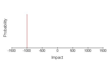
This is just part of the story of course. There is also the 0.9 probability of being paid by the insurance company as anticipated, whose impact might have been estimated at zero. The complete picture is, therefore, as below.
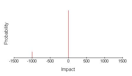
Provided the number of impact levels involved is small it is possible to characterise this type of distribution conveniently by listing or tabulating the impacts and their probabilities e.g. (-�1000,0.1), (0,0.9) However, as the number of impact levels gets larger this gets less attractive. This can happen with multiple-occurrence risks where the individual impact is fixed.
Another common distribution is a continuous variation of impact. For example, ‘Loss of market share’ will have different impact for each level of lost share. Imagine the probability of losing at least some market share is thought to be 0.5 and that greater losses are thought to be less likely according to this distribution:
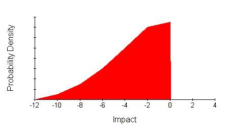
Instead of showing probability on the vertical axis this graph shows probability density, which is a mathematical concept that works like this: The red area covers 0.5 units. That means the probability of losses between zero and -12 is 0.5. The probability of losses between any pair of loss levels in this range is the area under the curve between those two levels.
This sort of distribution might be characterised in a few numbers by saying the likelihood of a loss greater than some other number, or by showing the whole distribution.
(An alternative is to slice the range of the variable into zones and then behave as if the distribution was a set of discrete values instead of being continuous).
Once again this is not the full picture. What about gaining market share or holding it? The full picture might look like this.
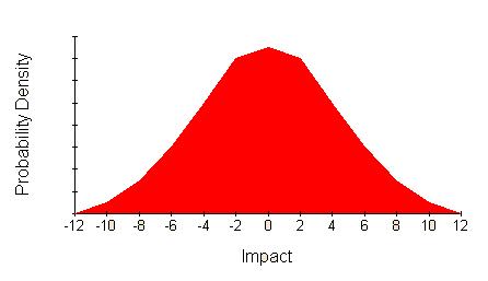
This distribution is symmetrical and broadly bell/triangular shaped. A common way to characterise such a distribution is using its mean value (the centre) and variance (how spread out it is).
However, this can be misleading if the distribution is skewed, like this:
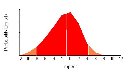
The upside has been squashed down so using mean and variance is not appropriate. This type of distribution might be characterised by giving the levels of impact such that you are 10%, 50%, and 90% certain that the impact will be less, or by showing the whole distribution. On the above picture the 10% and 90% levels are picked out in sticking plaster pink and the 50% level with a white line just to the left of the peak.
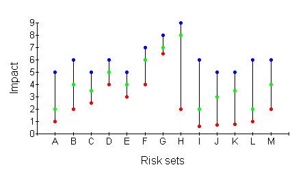
A number of distributions characterised by three numbers (or more) like this can be summarised using a Tukey box-and-whisker plot, or something similar like this:
Not all continuous distributions have attractively hill-like distributions. Some look more like mountain ranges.
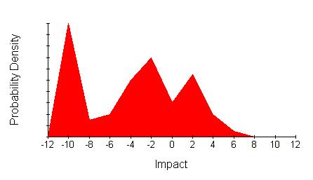
This is very difficult to characterise without being misleading unless you show the whole distribution.
There are also many risk sets which are hybrids. For example, ‘Risk that Tiger Woods pulls out of our tournament’ may have a probability estimated at 0.2, but the impact is not one number. His impact on the tournament may be hard to judge and past history may show that it is variable. So we need a discrete probability of 0.8 for his appearing as we expect (impact zero by our choice of baseline) and a continuous distribution for the loss if he doesn't show.
Imagine you are looking at one or more risk sets on a risk register and need to decide how to characterise them. Should you do it by showing the full picture, or choose some summarising numbers? It depends on how much time and skill you have, and how much it matters to be precise. If you're not going to show the full picture, your method of characterising depends on the overall shape of the distribution. Even if you are going to show the full picture you need a variety of methods to accommodate discrete, continuous, and hybrid distributions.
If all the risk sets in the register have similar distribution shapes it may be possible to use the same method of characterisation throughout. Otherwise this is not going to work very well.
(Technically, it is possible to describe all of these distributions using one type of graph: the cumulative probability density function. This is a graph with impact along the bottom and probability on the vertical axis. The line shows the probability that the impact is less than or equal to the impact at that point. The lines start near the bottom left of the graph and slope up towards the top right. Technically this is fine, but in practice it is hard to read these, which limits their use.)
The quickest and dirtiest method is always to get people to just rate or rank the risk set for ‘importance’ with no analysis or helpful characterisation of the shape of the distribution. The most comprehensive method is always to show the full distribution. An alternative with any continuous distribution is to slice it up and pretend it is a set of discrete impact levels. Here's a summary of the other options:
Distribution shape | Alternative rating forms |
|---|---|
Small number of discrete impact levels. |
List each impact level and its associated probability. |
| Large number of discrete impact levels. | Consider approximating it as a continuous set, and treat appropriately (see below). |
One half of a bell shaped curve (might be symmetric or skewed). |
One or more pairs of numbers each meaning ‘I'm X% sure the impact will be no more than Y.’ |
A symmetric curve of roughly bell or triangular shape |
Mean and variance. |
A skewed bell/triangle shape |
Pick some levels of confidence (e.g. 10%, 50%, and 90%) and state the level of impact for each such that you are that sure the impact is no more than the level. |
A mountain range |
No good options. |
A hybrid of a small number of discrete impact levels and a continuous distribution that is symmetric and roughly bell shaped |
List each discrete impact level and its associated probability level, plus the probability of the result being in the continuous distribution. Then characterise the continuous distribution using mean and variance. |
A hybrid of a small number of discrete impact levels and a continuous distribution that is skewed but roughly bell shaped |
List each discrete impact level and its associated probability level, plus the probability of the result being in the continuous distribution. Then characterise the continuous distribution using impact levels for a small number of confidence levels. |
A hybrid of a small number of discrete impact levels and a continuous distribution that looks like a mountain range |
List each discrete impact level and its associated probability level, plus the probability of the result being in the continuous distribution. Then sketch the mountain range. |
Using expected values
Comparing two distributions can be difficult. One way is to calculate the Expected Value (EV) of a set of risks. For example, the EV of a risk whose probability is 0.1 and whose impact would be �1,000 is �100 (i.e. 0.1 x �1,000). If the risk set has, say, three risks in it the EV is the sum of the EV of each risk. (There is an analogous definition for continuous variables based on probability densities.)
Converting distributions into expected values condenses the information and tells you what to expect ‘on average’. However, it throws away the very thing you are trying to capture – the risk. As soon as you stop representing uncertainty explicitly in your modeling the true nature of risk is out of view and the Flaw of Averages threatens to undermine the accuracy of your calculations. The same is true when, instead of probability, average frequency of occurrence is used. This is almost an expected value in disguise.
Try to avoid using expected values, except when comparing distributions of the ultimate impact of risks expressed as utility.
Using utility is, in theory, acceptable. Although humans do not behave quite in accordance with the recommendations of utility theory, one of the leading explanations for risk being undesirable is that we tend to value our last �1 much more than our millionth. Offered a bet with a risk of losing �100 and an equally likely risk of gaining �105 most people turn down the bet. This is quite rational if your utility for �100 lost is greater than your utility of �105 won.
Backing up distributions
Providing risk ratings that are more than unreliable guesswork usually requires a lot of careful work. What is the best approach? How much is appropriate? Is it necessary to go to the same lengths for every risk set on your risk register? You might try to make a choice that applies to every risk, or decide your approach for each risk individually, or make a policy that says when certain techniques should be used. In this section I'll run through some things you can vary and consider reasons for choosing one approach over another.
The importance of the application
Is it a matter of life and death or just some money, and if so how much? How important is the risk assessment to the decisions involved? This can be considered for the whole exercise and for individual risks. Risks that clearly require action, or clearly don't, perhaps do not need to be examined in the same depth as risks that are not well known but could justify some expensive management actions.
Empirical support
All probabilities are judgments; but having data behind you gives a lot of extra confidence. Sometimes the element of judgment is not obvious. It may be just a judgment like ‘the FTSE 100 index will continue to wobble about tomorrow the same way it has in the previous year, so my estimate is this number my computer has calculated from the previous year's real data.’
Directness
One factor affecting the value of data is how directly it helps you get to the final answer. For example, suppose you want to estimate the distribution of impact for thefts affecting your company's vehicles in a year. The final answer needs to be a distribution of impact, but the available data may just show the number of incidents in each year, or each month. How helpful is this? It's vastly better than nothing but getting from there to the final answer is going to take some further guesswork and calculations, unless you can find some more directly relevant data.
Model complexity
As models, especially computer models, get more complicated and detailed they typically get more accurate – but not always. Small discrepancies between reality and parts of the model can accumulate and sometimes multiply within a large model, making it very difficult to establish whether it is working correctly and hard to track down problems when the model as a whole seems to be giving odd results.
Models based on many expert forecasts can sometimes be outperformed by simple statistical extrapolation, especially when the human forecasters are biased by motivation or normal human cognitive limitations. For example, statistical extrapolation of short term future sales distributions is often more accurate than asking all the sales people to submit estimates that are then added together. Not only is it more accurate, but also far easier.
Model availability
Many organisations already have models on computer but they do not show uncertainty explicitly. These ‘found models’ can sometimes be converted into models that represent uncertainty explicitly and tools like @risk, Crystal Ball, and XLsim help do this easily. Converting an existing model might also be a good choice if the existing model is already trusted.
Time period(s)
One important aspect of model complexity is the choice of time periods. One major advantage of simulating (e.g. Monte Carlo simulation) using a number of small time periods is that it is easier to build in the effects of decisions you might take in the future based on what has happened to that point. The value of taking decisions later with the advantage of more information is often huge.
Combining information by judgment or calculation
Wherever you have to combine information to make progress towards the final impact distribution there is a choice between doing it with maths and using judgment. If maths can be used then use it. Judgmental combination is notoriously inaccurate so that even very crude mathematical rules for combining information usually perform better.
Care over subjective estimates
You also have choices to make when obtaining subjective estimates by just asking people. Subjective estimates are notoriously prone to a range of biases, including some that almost defy belief because they are so stupid (e.g. anchoring induced by spinning a roulette wheel). For more on these biases see ‘Straight and crooked thinking about uncertainty’.
The main lesson from extensive research on how to elicit subjective probabilities is that it is extremely difficult, and doing it properly usually takes quite a long time. For example, here are the 5 stages of the Stanford/SRI Assessment Protocol, with explanations of why each is necessary. You can imagine from this description that care is needed and that the ratings on most corporate risk registers do not benefit from such care.
Phase 1: Motivating. There are two activities in the Motivating phase. One is to develop some rapport and discuss the basic idea of probabilistic assessment, explaining and justifying it. The other is a systematic search for motivational bias i.e. any reason why the expert might say something that does not represent his/her true beliefs. The importance of motivational bias varies greatly depending on the problem and the field.
Phase 2: Structuring. The objective of this phase is to arrive at an unambiguous definition of the quantity to be assessed, stated in the form in which the expert will be most able to provide reliable judgments. Careful work may be needed to unearth unspoken assumptions the expert may be making but which are not actually stated in the problem. The expert should not need to do units conversion or other mental acrobatics to provide the assessment required.
Phase 3: Conditioning. The objective of the conditioning phase is to get the expert ready to think about his/her judgment and avoid cognitive biases. The expert has to talk about how he/she will go about making the judgment, what data will be used, and how. Alternatives should be discussed while the analyst looks carefully for possible cognitive biases so that a method is arrived at that minimises them. Some researchers have taken experts through warm-up exercises to teach them about cognitive biases.
Phase 4: Encoding. In this phase the expert finally gives his/her assessments. Problems arising at this stage may indicate a need to go back to previous phases. Various methods can be used. When asking for the spread of some variable the common bias is for experts to give a spread that is too narrow. The analyst can counter this to some extent by first asking the expert to choose extreme values, and then asking the expert to describe conditions that might lead to results outside those extremes. The expert then gets the chance to think again.
Phase 5: Verifying. The objective of the final phase is to verify that the assessments obtained truly reflect the expert's views. Their ratings can be graphed and discussed with them. Probability statements can be constructed from the distribution to see if the expert agrees.
(Frequentists disagree with the previous paragraph, but if you are a frequentist please don't write. I know.)
The cost of getting relevant, reliable data is very different in different situations and this is a major factor in deciding how to back up estimates and to what extent it is possible.
Eliciting ratings is so time consuming to do properly that it may be worthwhile avoiding proper ratings for risk sets that are clearly key ones, or clearly trivial, and only doing ratings for risks that people want to think about more.
Risk identification alternatives
Risk identification is the first thing to be done, but it is not the first thing to design. The best way to identify risks depends on what you will do with them so has to be designed last.
For example, risk rating that focuses on losses is often supplied with risks by identifying an organisation's assets and listing the ways those assets could be damaged or otherwise become less valuable. Risk modeling based on cause-effect models tends to determine the risks; they are the distributions of the independent variables in the model, though it is also possible and desirable to adapt the model to incorporate other specific risks identified by other means.
Here are some considerations for designing the risk identification method:
Partitioning: Whatever risk identification method is chosen it is usually good to do it in a way that slices up risks so that everything is caught, but only once. There should be no gaps and no double-counting. The breakdown usually takes more than one level. For example, first by geography, then by business activity, etc. There is a big difference between having a list of areas to consider and having a list of areas to consider that is complete. Even taking a list of risk types from an official document such as a risk management standard does not guarantee that the list is comprehensive, but there are ways to think through the breakdown that guarantee completeness.
Relative entropy: It is also good to break down large risk sets so that all risk sets carry about the same amount of risk. This means management reports of risk are more informative per page than they would be if very large risk sets were not broken down and instead tiny risk sets were given space for their trivial statistics. This implies some risk assessment is needed during risk identification.
Clarity of objectives: A popular approach among internal control experts is to derive risks from business objectives. Risks are simply the ways in which you could fail to achieve your objectives. Unfortunately, life doesn't always allow clear objectives. Looking at risk is part of forming objectives, so you often need to do it before objectives have been set. Objectives are often unclear and shifting for very good reasons; if they did not move for a year it would imply an extraordinarily stable business environment or managers who have stopped thinking. Risk management needs to be able to ride this out so if there is any doubt about business objectives they should not be the sole basis of risk identification.
Volunteering: If you rely on people to volunteer risks they may not volunteer all the risks they know about. They may keep quiet because they don't want to risk offending senior management (or other groups they fear such as human resources and IT) or fear being made responsible for a risk about which little can be done. For risks where this is likely it may be necessary to put the risk into the register at the start and make rating dependent on objective criteria. For example, people may be reluctant to suggest ‘fraud by senior management’ as a risk, and even more reluctant to opine that the risk is high.
Richness: Some methods of risk identification tend to lead to bland, unhelpful risks and little if any insight. Taking your objectives as the source of risk ideas can lead to risks that are just the original objective with the words ‘Risk that we fail to’ stuck on the front. They also tend to be inward looking with the external environment ignored. Taking risks as just the independent variable in existing business models also leads to sterile risks.
Seven real examples
The following examples illustrate the astonishing variety of alternatives approaches to risk modeling for a risk register. They were chosen by searching the Internet for complete examples that illustrated variety and could easily be visited by readers with Internet access. Inclusion does not necessarily imply the method is a good one. Here is a summary.
Example |
Characteristics |
|---|---|
A new focus for Turnbull compliance |
The main purpose is to maintain sound internal controls. Risk is just one factor in decision making. |
| Integrated Risk Assessment | This is enterprise wide but focuses on mishaps. Centralised, downside-only, using expected values, independent risks. |
Opportunity And Risk System |
Primarily about project risks. Centralised, upside too, action oriented. |
@RISK in Procter & Gamble |
Widely applied tool used in a variety of applications. Partly decentralised, upside too, integrated models. |
P&C RAROC |
Typical financial services industry modeling approach. Centralised, upside too, Value at Risk based, highly mathematical and done by experts, limited to high level decisions. |
Structural modeling |
Aimed at all types of risk, and enterprise wide. Centralised, upside too, modeling an integrated system, fairly mathematical and done by experts, good for a variety of decisions including operational risk management. |
Mark to Future framework |
Alternative means of modeling linked risks, highly mathematical and done by experts, centralised, upside too. |
A new focus for Turnbull compliance
The Combined Code on corporate governance that regulates companies listed on the London Stock Exchange, and the ‘Turnbull guidance’ that interprets its requirements on internal controls, both emphasise evaluation of internal controls effectiveness. Risk assessment is a key part of that approach and of the internal control system envisaged. Consequently, much effort has gone into risk workshops and risk registers.
However, the real goal is to have better controls. By concentrating on that rather than evaluation companies can have better controls, meet evaluation requirements, and not spend extra money. Rather than making risk assessment and management more sophisticated to fix the technical flaws common in these exercises, it is better to simplify them further in most cases and concentrate instead on anticipating the need for internal controls development work.
This anticipation of controls work should be based on a number of factors and take into consideration not just risk, but also economic factors, the time needed to implement controls, and cultural fit. By surveying trends, plans, past omissions, control performance statistics, and so on, the top team can identify in advance where extra work is needed to build new controls or remove old ones.
Although risk analysis can be quite sophisticated at the detailed level of designing key controls the process for senior directors (e.g. formed into a Risk and Control Committee) is a more familiar one of approving the direction of resources to meet anticipated needs.
A method of doing this is explained in my paper ‘A new focus for Turnbull compliance’.
Integrated Risk Assessment (IRA) by ABS Consulting
Integrated Risk Assessment by ABS Consulting was offered as an enterprise wide risk assessment approach. Although it aims to cover an entire enterprise it does not cover all types of risk. This approach is aimed at mishaps, so the risks have only downsides. Great accuracy is not claimed and risks appear to be considered independent of each other.
First, the types of mishap to be considered are listed. The enterprise is broken down in stages by some means, such as by geography, then activities, sub-activities, etc to make a hierarchy.
Risks/risk sets are rated by identifying three levels of impact for each: Major, Moderate, and Minor (all with numerical ranges to define them in cost terms). This is a simplification compared with a continuous impact distribution but far better than ignoring the variation in impact.
This generates a matrix with a row for each type of mishap and a column for each level of impact. For each cell in this matrix, average long run frequencies are estimated. (In effect there is no attempt to capture the uncertainty about how many incidents happen per period.)
Risk scores can be used in various ways. One is that the impact ranges are given ‘average’ impact values which are multiplied with the frequencies to give annualised costs. The annualised cost for risk sets can be aggregated up the hierarchy of activities/locations/etc to give overall scores.
Opportunity And Risk management in BAE SYSTEMS Astute Class Limited
Whereas ABS Consulting's Integrated Risk Analysis looks only at downside risk, BAE SYSTEMS Astute Class Limited (ACL) used an approach that included potential opportunities too. The company was set up in 1997 as an independent company within GEC Marconi to manage work on nuclear submarines for the UK Royal Navy. Its approach has been applied to its projects and to the company itself. A software tool, Opportunity And Risk System (OARS), has been used, run over a secure WAN with terminals at participating sites.
Although the description of this approach makes many references to published standards the system of ideas used in OARS is unusual. Here's how the thinking works. I've picked out key terms in italics.
The starting point is a set of requirements, reflecting all stakeholder views. This is examined to identify potential effects, i.e. areas in the outcome that could be affected by risks or opportunities to the business or project. The requirements also allow construction of a solution, i.e. a design specification and plan to meet the requirements (e.g. design and plan to build a nuclear submarine). The solution gives rise to a set of baseline assumptions about the solution from which issues will arise. Issues that remain unresolved become the causes of risks or lost opportunities. Issues can be resolved by taking timely action. If action is successful it will reduce the probability of risks occurring and/or enable opportunities to be realised.
In OARS risks and opportunities are opposites. Risks are bad things that might happen and need to be mitigated and made less likely, whereas opportunities are good things that might happen and need to be realised and made more likely. ACL also refers to uncertainty as other things that might happen and affect achievement of objectives, but which have not been identified specifically as risks or opportunities.
However, ACL may not have fully balanced their thinking about risk and opportunity. They say that many opportunities have been included in bids on the assumption that they will be realised. They point out that this approach gives the risk that the assumption is unrealistic and the benefits will not be realised. Either realising these opportunities is in the baseline assumptions, in which case ACL's risk and opportunity management system is not a truly balanced one, or they are outcomes better than the baseline and it is optimistic bidding that is at fault.
[It could well have been the bidding that was at fault. The paper I am relying on for this description was written in 2001, long before a huge row erupted between the UK government and BAE SYSTEMS about cost overruns on the Astute submarines and another project. The government felt that BAE SYSTEMS should pay for the entire �800m overspend.]
In addition to ACL's system of concepts their approach has some other interesting innovations.
To help people categorise their ideas according to the OARS concepts they prompted people to start sentences with standard words that would tend to elicit the right kind of concept in response. For example, a sentence that has to start with the words ‘The risk is caused by...’ is likely to prompt a cause for a risk.
Also, since the thinking required to model risks etc could not be done quickly enough for a group brain storming exercise they developed a simpler form of workshop based on identifying worries and wishes. These tended to collect a mixture of issues, sources of risk, opportunity actions, and effect/benefit areas. Once collected these were then analysed into the structure needed by OARS.
Risk and opportunity workshops were held at four levels:
Level 1: ACL Business level: Quarterly meetings chaired by the managing director and attended by all directors, to manage business issues and actions at a strategic level.
Level 2: Project level: Quarterly meetings chaired by a project director and attended by appropriate directors and senior managers, to manage project issues and actions.
Level 3: Sub-project level: Monthly meetings chaired by the relevant director/senior manager, to reconcile the top down view of the higher level meetings with the bottom up view of lower level meetings. These workshops also managed the more severe specific risks, important opportunities, and associated actions.
Level 4: Functional area level: Monthly meetings chaired by the relevant functional director or senior manager and attended by the owners of specific risks, opportunities, and actions, to manage the detail as required by level 3 workshop chairmen.
In smaller projects levels 2 and 3 were combined into a single meeting. Top down brainstorms were held at all levels at major project/business milestones.
Use of @RISK and PrecisionTree in Procter & Gamble
@RISK is a software tool much like a conventional spreadsheet that adds Monte Carlo simulation and related tools to models that would otherwise typically work on the basis of best guesses.
According to Palisade, the company that sells the @RISK and PrecisionTree software tools for modeling risk and decision making under uncertainty, their customer Procter & Gamble uses @RISK worldwide for investment analysis and over a thousand employees have been trained to use it. The company has used the tool for decisions including new products, extensions of product lines, geographical expansion into new countries, manufacturing savings projects, and production siting.
It was first used by the company to model production siting decisions in 1993. The decisions involved taking into account uncertainties involving the capital and cost aspects of the locations, and also exchange rate fluctuations for cross-border sites.
Similar software is offered by Crystal Ball, and AnalyCorp, among others.
P&C RAROC
A very different approach is described by Nakada, Shar, Koyluoglu, and Collignon for application to Property and Casualty (P&C) insurers. Their approach has many features typical of financial risk modeling.
Their model tries to estimate how strong a P&C insurer's balance sheet has to be at the start of a financial period to reduce the risk of business failure during the period to some specified level. The value of the balance sheet is measured in terms of its net realisable value, because if the company folds that's all you get.
Having answered this question for the business as a whole they go on to apportion the value needed for each business activity so that the cost of that capital can be considered when evaluating the contribution of each activity. Some business activities will be found to provide a good return for the capital required and the uncertainty of the activity's returns (i.e. a good Risk Adjusted Return on Economic Capital – RAROC), while others will be found disappointing.
Rather than involving management in workshops, this kind of risk modeling is done by experts using statistics, computers, and more mathematical skill than most people would like to think about. Rather than using simulations they have used mathematical formulae, fitted to data where possible. This means their model runs quickly on a computer and gives precise answers for extreme risks, but some realism has been sacrificed in the model.
The steps of their procedure are:
Generate distributions for each risk category in isolation. They have 6 risk categories within three broad risk types:
- asset risk – credit, and market;
- liability risk – catastrophe, and non-catastrophe; and
- operating risk – business, and event.
Calculate economic capital for each risk category in isolation.
Aggregate risk categories taking into account correlations between risks and calculate the economic capital needed for the business as a whole. (This will be less than the sum of the individual risk categories because of the diversification effect.)
Allocate the diversification benefit back to risk categories (on the basis of their contribution to the total economic capital) to arrive at revised economic capital estimates for each category. Now the sum of the economic capital for all categories is the same as the total economic capital for the business.
Calculate risk adjusted return on capital for activities.
The risk categories have been chosen on the basis of their risk drivers and distribution shapes. Different techniques are used to model risk in each category:
Risk category |
Definition |
Approach to modeling |
|---|---|---|
Credit |
Variability in losses arising from debtors failing to pay, either because they cannot or will not. Key exposures are reinsurance recoverables and corporate bonds. |
The distribution type is skewed (low frequency, high severity) and can be modeled by an options formula, a predictive formula using macroeconomic variables, or by fitting curves to actual loss history. |
| Market | Variability from changes in market value of securities. Key exposures are equity investments and asset/liability mismatch (interest rate risk). | Modeled assuming normally distributed returns and lognormal asset prices, and a portfolio of securities with correlated random price movements. The price movements are the result of risk factor movement and risk factor sensitivity. In translating VaR to economic capital they used a confidence level of more than 99.9% and consider the changes to VaR through the year, autocorrelations of daily returns, and economic effects of possible management decisions in response to changes in portfolio value. |
Catastrophe |
Variability in losses from natural disasters like hurricanes, tornadoes, floods, and earthquakes. Key exposures are the catastrophic elements of property lines. |
Highly skewed distribution. Because historical catastrophe data is limited, catastrophe risk was modeled on a computer using various analytical, engineering, and empirical techniques, relying on established principles of meteorology, seismology, wind, and earthquake engineering, and related fields. |
Non-catastrophe |
Variability in the amount and timing of insurance claims – excluding catastrophe. |
Modeled in various ways, but generally close to lognormal. The method relies on characterising the amount and timing of future claims by statistical analysis of past claims. |
Business |
Variability due to fluctuations in volumes and margins driven by the competitive environment. |
Modeled by normal distributions. Pricing risk is based on measurements of past volatility in pricing adequacy, and volume risk is based on past volatility in premium volumes. |
Event |
Variability in losses caused by events such as fraud and systems failure. |
Modeled by Poisson event frequencies with exponentially distributed severity, fitted to actual loss data from other companies in the financial services industry. |
Structural modeling (mainly for operational risk)
An alternative to the statistical correlation method of aggregating risks is ‘structural modeling’, described by Jerry Miccolis and Samir Shah. Structural models simulate the dynamics of a specific system by modeling cause-effect relationships between variables in that system. Various techniques can be used including stochastic differential equations (useful for financial risks), system dynamics, fuzzy logic, and Bayesian networks.
A wide range of macroeconomic risks can be modeled as a cascade structure where each variable is dependent on the variables above it.
One structural method is system dynamics simulation. The starting point is to use experts' knowledge to diagram the cause and effect relationships of interest. Then, each cause-effect relationship is quantified using historical data and expert judgment. If there is uncertainty the cause-effect relationship is represented by a probability distribution around a point estimate.
The simulation is run to find the ranges of operational and financial variables and the output can be summarised as a probability distribution for financial variables. Alternative operational risk management actions can be evaluated by modifying the model and running what-if analyses.
Mark to Future modeling
The Mark-to-Future (MtF) framework offered by Algorithmics offers an alternative to statistical aggregation of risk using correlations. Algorithmics claim it has performance advantages as well as being easier to understand.
In conventional statistical modeling of risk in, say, a portfolio of shares you need to know the portfolio and the correlations between returns from shares in each company. In the MtF approach you do not need to know the portfolio before doing most of the intensive computations.
To use this approach you need to:
choose the securities you might want to model;
produce a (large) set of scenarios showing how key variables in the financial environment might change over future time periods; and
define pricing functions that give the price of each security (and other numbers about it such as dividends) in each time period given the state of the financial environment specified in each scenario for that time period and perhaps previous prices.
All the probabilistic aspects are captured in the scenarios.
Once the system has calculated the prices etc of all securities in every time period for all the simulated scenarios it is relatively easy to find the value of different portfolios at different times. The probability distribution of the value of a portfolio at a particular time is the distribution of the sum of the prices of the individual stocks under each of the scenarios. It is also relatively easy to do more sophisticated calculations to examine different management policies.
Conclusions
The variety of alternative theories about risk and methods for modeling and managing it is extraordinary. There are more variations than most people realise.
In this paper I have discussed alternatives for modeling risks for a risk register, but much valuable risk management can be done without a risk register. For example, decisions can be made on the basis of areas of uncertainty existing, without any more detailed analysis, and internal control systems can be designed as integrated systems rather than by working out responses to each risk individually. Also, although I mentioned informal, decentralised risk management I said very little about it.
Before designing a system for your own use it is vital to open your mind to the range of options.
Further reading
Relevant publications by Matthew Leitch include:
The 7 examples were based on the following:
@RISK case studies reported on the Palisade website.
‘Enterprise Risk Management’ by Vernon Guthrie and David Walker of ABS Consulting and Bert Macesker of the United States Coast Guard Research and Development Center. (Unfortunately you have to register before they send you the article but it is very quick.)
‘Modeling the Reality of Risk: The Cornerstone of Enterprise Risk Management’ by Jerry Miccolis and Samir Shah of Tillinghast-Towers Perrin, and appearing on the IRMI website.
The Algorithmics website and its various papers about the Mark to Future framework.
‘Implementation of Opportunity & Risk Management in BAE SYSTEMS Astute Class Limited – A Case Study’ by Andrew Moore, Alec Feardon, and Mark Alcock. This seems to be unavailable online now, but similar information is given in their ‘Implementation of Opportunity & Risk Management in BAE SYSTEMS Astute Class Limited: A Case Study’
‘P&C RAROC: A Catalyst for Improved Capital Management in the Property and Casualty Insurance Industry’ by Peter Nakada, Hemant Shah, H. Ugur Koyluoglu, and Olivier Collignon, of Risk Management Solutions.
Other interesting software tools are available:
The Analytica modeling software system.
Crystal Ball is a spreadsheet add-in similar to @RISK
XLsim software is another Excel add in. Though far less sophisticated than @RISK and CrystalBall it is cheap and comes with a brilliant tutorial by Dr Sam Savage. This is a superb educational opportunity and the software is quite capable of professional modeling.
Sawtooth are the leading vendors of conjoint analysis software.
However, a great demo of conjoint analysis is provided by Saul Dobney.
Appendix: The terms ‘rate’, ‘assess’, and ‘quantify’
In this page I use the terms ‘rate’, ‘assess’, and ‘quantify’ as if they all meant the same thing but many people draw distinctions. The words have slightly different connotations and are usually seen in different settings:
‘Rating’ is usually used for things like hazardous chemicals or the credit worthiness of companies. The rating could be a number or some other code but it is an invented variable rather than something like probability, money value, or utility. Rating is usually used in situations where there are lots of similar things to be rated and their risks are not really linked. Rating is often done using a formula of some kind that gives points for having certain attributes. For example, a chemical that is toxic, explosive, corrosive, and gaseous at room temperature would get lots of points that plain water does not.
‘Assessing’ is usually used for attempts to say how much impact something is likely to have, but that stop short of probability or value numbers. For example, they might say that the impact is ‘High’, or that it is ‘3’ on a scale of 1 to 5.
‘Quantifying’ is sometimes reserved for statements that are made in terms of probabilities and values of impact. ‘Quantification’ suggests a more rigorous, precise, and time consuming procedure than ‘assessment’.
This page is about all these kinds of activity.
Made in England