Working In Uncertainty

Why is Evolutionary Project Management so effective?

by Matthew Leitch, first published 25 July 2003.

Evolutionary Project Management

Why is Evolutionary Project management (EPM) so much better than a conventional waterfall? This document suggests some reasons and illustrates them with very simple calculations.

But first, what is Evolutionary Project Management, and how do we know it is better than conventional waterfall methods?

Evolutionary Project Management, as described by Tom Gilb (one of the key figures in this area) is characterised by several principles. However, two in particular are distinctive: (1) it involves incremental deliveries – about 50 of them; and (2) the specific objectives evolve as things are learned during the project. In Gilb's approach progress on ‘performance characteristics’ of interest to stakeholders is the focus for planning and prioritising deliveries.

Evolutionary Project Management is particularly advantageous in conditions of risk and uncertainty, but even in relatively stable situations it is superior.

A case study has been written by Stuart Woodhead, an IT project manager who had the experience of managing two nearly identical projects, one of which was a failure using conventional methods, the other being managed with evolutionary methods with great success. The case study (sadly no longer available online) is a very realistic description of these methods as used on a small scale.

The Standish Group have carried out extensive research on thousands of IT projects to find out what factors are linked with success and failure. They have concluded that early and frequent delivery of useful outputs, as in evolutionary methods, is the best approach. One of the major reasons for this is that there is a dramatic relationship between project size and success rate, and an evolutionary project is, effectively, a series of small projects. Evolutionary methods also score well on other factors the Standish Group believes to be linked with project success: user involvement, clear business objectives, small milestones, and ownership.

Illustrations of advantages

If you're not familiar with EPM you may be thinking ‘How can 50 releases be more efficient than 1?’ There is indeed an overhead from slicing a project up in this way. There's some extra thought and work needed to get into a position where 50 deliveries can be done efficiently, and there's a small overhead with each delivery. The skill of the EPM expert is in minimising these overheads. I have not analysed the overheads in this paper but work by others to be published shortly will show that they are more than covered by the advantages, even on projects with low uncertainty.

To explore the reasons for EPM's effectiveness I've constructed some simple mathematical models of the major effects that may affect a project's expected value, and created graphs linking these effects to the number of deliveries in a project. Generally, the more the project is sliced up into smaller deliveries the better.

Although the models are very simple and some big simplifying assumptions have been made, on the major estimates you can make up your own mind about how strong you think the effect would be and see the effect on project value. The effects are usually dramatic even with conservative assumptions so it is easy to see that any drawbacks with EPM would have to be massive to offset the advantages.

Each model looks at one effect. In a real project these benefits would combine with each other.

You will see how delivering benefits as you go through a project is much better than waiting until the big bang at the end.

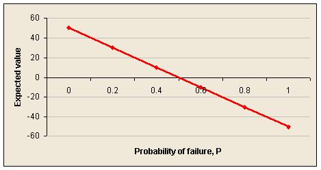
The effect of project failure

For this illustration imagine a project with overall benefits of B, and overall costs of C. The overall probability of the project failing is P, and in this project there is either total success or total failure.

Worst case – not evolutionary

First, imagine that the project is broken into N stages, that have to be completed successfully in sequence. If there is failure at any stage we don't know about it and continue with later stages. However, at the end if there has been any failure at all no benefits are achieved despite incurring the full costs.

In real life this is like a technically challenging waterfall project to build something that we can't test until it is all put together.

The expected value of a project structured and managed like this is independent of the number of stages, and decreases as the probability of failure increases:

EV_A = B.(1 - P) - C
[derivation]

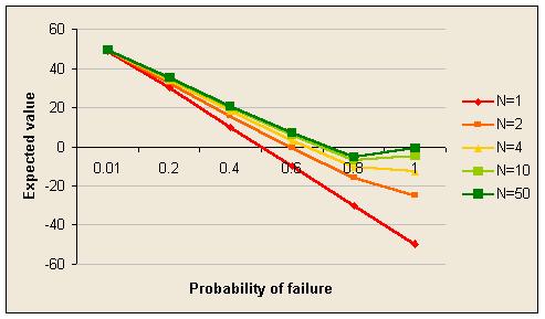
Ability to abandon – but still not evolutionary

Imagine a project similar to the first, but at least if a stage fails we will realise at the end of that stage and stop further work. This improves the position, a little.

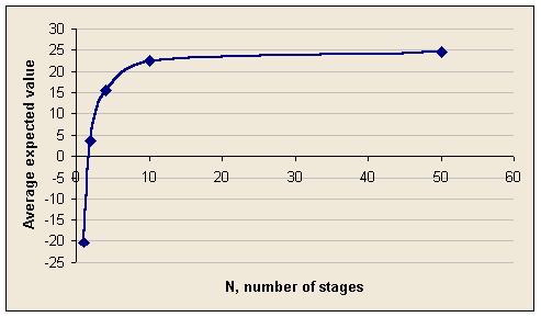
The expected value of a project structured and managed like this improves as the number of stages, N, increases:

EV_B = B.(1-P) - (C/N).( 1 - (1-P)]/(1 - (1-P)^(1/N))
[derivation]

Separate stages

Now imagine that the stages of the project are independent and each stage has a share of the benefit that is received when that stage is completed successfully, regardless of what happens on other stages. This is like a set of independent projects.

The expected value of such a project is the sum of the expected value of each stage:

EV_C = (1 - P)^(1/N).B - C
[derivation]

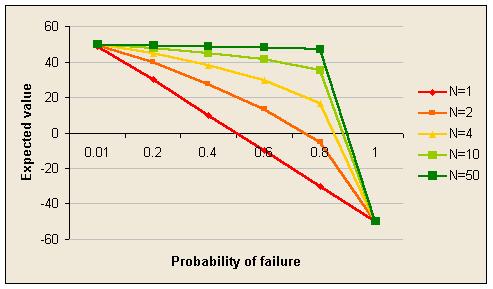
These graphs are dramatic. Sliced into 50 stages a project seems almost immune to the overall probability of failure in at least one stage. This is because the probability of failure on any one stage is low even when the probability of failure on at least one is high.

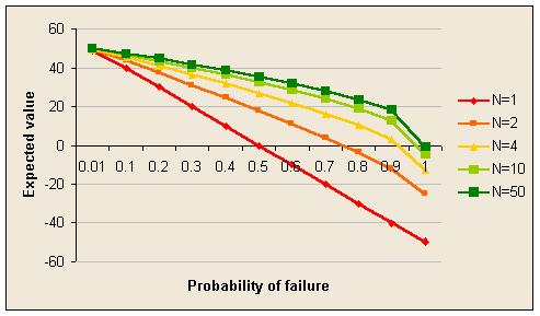
Evolutionary but in sequence

Now imagine that individual stages once again deliver benefit if completed successfully, but now they have to be done in sequence and if one stage fails the project stops.

The expected value of such a project is:

EV_D = [((1 - P)^(1/N).B - C).P)]/((1-(1-P)^(1/N)).N)
[derivation]

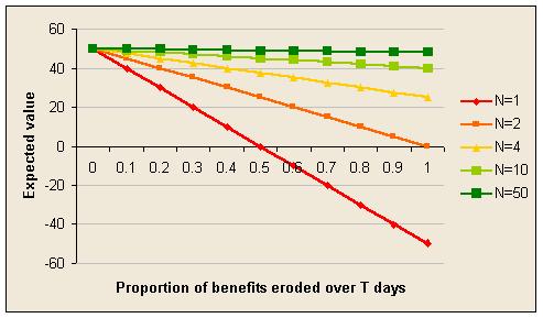
The effect of changing conditions

Another criticism of waterfall methods is that in a long project the original objectives become progressively out-dated.

Imagine a project with benefits B, costs C, and N stages taking in total T days to complete. Suppose there is no possibility of failure and benefits are delivered on completion of each stage, but the benefits of a stage depend on how long the stage takes to complete. The longer the stage the lower the benefits because of out-dated requirements.

Let's assume for the sake of illustration that the erosion of benefits is linear and that the proportion of benefits eroded after T days is E.

The expected value of such a project is independent of the overall duration T:

EV_E = B.(1 - E/N) - C
[derivation]

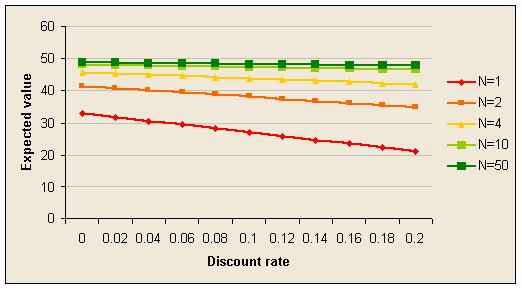
Effect of receiving benefits earlier

The preceding illustrations have assumed that it does not matter when benefits are received. But of course it does matter. First, there is the time value of money, usually modeled by discounting cash flows. Second, there is the fact that many projects are designed to improve some process and so produce regularly recurring benefits compared to the previous version of the process. The sooner the improvement starts the better.

In this illustration, failure and obsolete requirements are not a problem. The only factor is the timing of benefits. The interest rate for discounting is I per year (i per day) and benefits can be enjoyed until Y years after the start of the first stage. The total duration of the project is T days and it is assumed that the project finishes before the Y years are up.

The expected value of the project is:

EVF = (B/((1 - (1+i)^-Y.365).N)).[(1+i)^-T/N+1.(1 - (1+i)^-N)/i - N.(1+i)^-Y.365] - C
[derivation]

Where C is the NPV of project costs, and B is the NPV of benefits that could be achieved if all the process improvement was delivered immediately.

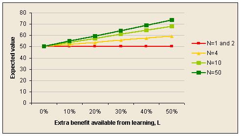
Effect of opportunities to learn

Having something delivered and operating live is a great source of ideas for improvements. The project team may have the ability to deliver a certain level of process improvement at the start of a project, but acquire the ability to deliver more if they have the opportunity to learn from real experience.

In practice, there are some problems that just cannot be solved without getting some experience to guide problem solving.

The expected value is:

EV_G = B.[1 + (L/(2.N²)).(N-2).(N-1)] - C
[derivation]

Where B is the benefit you think you know how to achieve at the start of the project and L is the percentage of extra benefit that would be available if you knew at the start everything you could learn from delivering the whole of the original project and learning from that experience.

There are many alternative ways to model learning effects and this is just one of the simpler ones. A more complex alternative is to assume that new learning lifts the benefits not from the original project, but from the project reached at the previous stage end. This increases the learning effect.

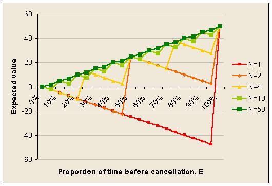
Effect of unexpected project cancellation

Suppose a project is unexpectedly cancelled before it is finished. In this illustration it is assumed that costs are incurred daily, but benefits are received only at the end of each completed stage.

As usual, the more stages there are the better. The expected value is:

EV_H = (B/N).int(E.N) - E.C
[derivation]

Where E is the proportion of the project time elapsed before cancellation and int() means the integer part of the number inside the parentheses.

Appendix: derivations of formulae

Worst case scenario

Assume that the sub-stages are all identical in cost and probability of failure.

The overall probability of failure, P, is related to the probability of failure in any one stage, p, by this equation:

(1 - P ) = (1 - p)^N

where N is the number of sub-stages.

A manipulation of this that we need later on is:

p = 1 - (1 - P)^(1/N)

For the project to succeed overall, each stage has to be completed successfully so the expected value is:

EV_A = B.(1 - p)^N - C

Or, alternatively:

EV_A = B.(1 - P) - C

Ability to abandon

In this project structure the expected benefits are the same, but the expected costs are generally less because of the ability to avoid wasting money on stages after a failure.

Again, assume that every stage is the same, so that the cost of each stage is C/N. The expected cost is the sum of the expected cost of failure on the first stage, second stage, etc plus the expected cost if no failure at all.

Expected cost = (C/N).( 1.p + 2.(1-p).p + 3.(1-p)².p + .. + N.(1-p)^N-1.p + N.(1-p)^N)

To find the sum of the middle terms, denote them by S, and use the usual trick for working out geometric series:

S = 1.p + 2.(1-p).p + 3.(1-p)².p + .. + N.(1-p)^N-1.p

S - S*(1-p) = 1.p + (1-p).p + (1-p)².p + .. + (1-p)^N-1.p - N*(1-p)^N.p

Therefore:

S.p = 1.p + (1-p).p + (1-p)².p + .. + (1-p)^N-1.p - N*(1-p)^N.p

S = 1 + (1-p) + (1-p)² + .. + (1-p)^N-1 - N*(1-p)^N

Using the same trick again let

T = (1-p) + (1-p)² + .. + (1-p)^N-1

T.p = (1-p) - (1-p)^N

T = [(1-p) - (1-p)^N]/p

Substituting this back into the expression for S:

S = 1 + [(1-p) - (1-p)^N]/p - N*(1-p)^N

Then substituting this back into the expression for the expected cost:

Expected cost = (C/N).( {1 + [(1-p) - (1-p)^N]/p - N*(1-p)^N} + N.(1-p)^N )

Simplify slightly:

Expected cost = (C/N).( 1 + [(1-p) - (1-p)^N]/p )

Expected cost = (C/N).( [1 - (1-p)^N]/p )

Replacing the p terms with P terms gives:

Expected cost = (C/N).( [1 - (1-P)]/(1 - (1-P)^(1/N))

Which simplifies slightly to:

Expected cost = (C/N).( P/(1 - (1-P)^(1/N))

Finally, putting the expected benefit with the expected cost gives the expected value:

EV_B = B.(1-P) - (C/N).( 1 - (1-P)]/(1 - (1-P)^(1/N))

Separate stages

The expected value of such a project is the sum of the expected value of each stage:

EV_C = N.[(1-p).B/N - C/N]

Simplifies to:

EV_C = (1-p).B - C

Replacing the p term with a P term gives:

EV_C = (1 - P)(1/N).B - C

Evolutionary but in sequence

The total expected value is the sum of the expected value if failure occurs on the first stage, the second stage, etc plus the value if there are no failures. If a stage fails its cost is incurred but its benefit is not delivered.

EV_D = (p/N).[(0.B-C) + (1-p).(1.B - 2.C) + (1-p)².(2.B - 3.C) + .. + (1-p)^(N-1)((N-1).B - N.C)] + (1-p)^N.(B - C)

To find the sum of the series we can use the usual trick for geometric series again. Let

S = (0.B-C) + (1-p).(1.B - 2.C) + (1-p)².(2.B - 3.C) + .. + (1-p)^(N-1)((N-1).B - N.C)

S.p = -C + (1-p).(B - C) + (1-p)².(B - C) + .. + (1-p)^(N-1)(B - C) - (1-p)^N((N-1).B - N.C)

Which simplifies slightly to:

S.p = -C + (B - C).[(1-p) + (1-p)² + .. + (1-p)^(N-1)] - (1-p)^N((N-1).B - N.C)

Using an earlier result for the sum of the series remaining

S.p = -C + (B - C).[(1-p) - (1-p)^N]/p - (1-p)^N((N-1).B - N.C)

Substituting this back into the expression for the expected value gives:

EV_D = (1/N).[ -C + (B - C).[(1-p) - (1-p)^N]/p - (1-p)^N((N-1).B - N.C)] + (1-p)^N.(B - C)

More simplification is possible:

EV_D = (1/N).[ -C + (B - C).[(1-p) - (1-p)^N]/p - (1-p)^N((N-1).B - N.C) + (1-p)^N.N.(B - C)]

EV_D = (1/N).[ -C + (B - C).[(1-p) - (1-p)^N]/p + (1-p)^N.B]

EV_D = (1/N).[-C.p + B.(1-p) - C.(1-p) - B.(1-p)^N + C.(1-p)^N + p.(1-p)^N.B]/p

EV_D = (1/N).[-C.p + B - B.p - C + C.p + (1-p)^N.(-B + C + p.B)]/p

EV_D = [B.(1 - p) - C + (1-p)^N.(C - (1 - p).B)]/(p.N)

EV_D = [( (1 - p).B - C).(1 - (1-p)^N)]/(p.N)

Replacing p terms with P terms gives:

EV_D = [((1 - P)(1/N).B - C).P)]/((1-(1-P)^(1/N)).N)

Linear erosion of benefits due to the duration of stages

Here's how the erosion of benefits is modeled. Suppose the maximum benefit a stage could achieve, by completing instantly, is b, and the stage takes t days. The benefit delivered is b.(1 - E.t/T), where T is the total project time and E is the proportion of benefits lost over T days.

The expected value for the project as a whole is the sum of the expected values of each stage.

EV_E = N.((B/N).(1 - E.(T/N)/T) - C/N)

Which simplifies to:

EV_E = B.(1 - E/N) - C

Time value of money and benefits of earlier process improvements

The annual interest rate is linked to the daily interest rate as follows:

(1 + i)³⁶⁵ = (1+I)

Which implies:

i = (1 + I)^(1/365) - 1

All benefits will be translated into a Net Present Value as at the start of the project. Completing a stage brings a benefit that recurs daily until the Y year horizon is reached. Total project duration is T days. Y is large enough that the project always finishes before Y is reached.

In this illustration, B represents the maximum possible benefits assuming the project is completed instantly. This arises from an improvement in process performance worth D per day.

B = (D/i).(1 - 1/(1+i)^Y.365)

Which implies:

D = B.i/(1 - (1+i)^-Y.365)

Each of the N stages of the project, once completed, delivers daily improvement of D/N.

In this illustration C represents the NPV of the costs of the project and do not change.

Suppose a daily improvement of d is delivered at the end of t days. Daily benefits are enjoyed at the end of each day. The NPV as at the start of the project of that daily improvement delivery is:

NPV = d/(1+i)^t.[1/(1+i) + 1/(1+i)² + .. + 1/(1+i)^Y.365-t]

= d/(1+i)^t .[1 - (1+i)^t-Y.365]/i

= [(1+i)^-t - (1+i)^-Y.365].d/i

The NPV of the benefits delivered by the project equals the sum of the NPV of the benefits delivered by each stage.

Expected benefits = (D/(N.i)).[(1+i)^-T/N - (1+i)^-Y.365) + (1+i)^-2.T/N - (1 + i)^-Y.365 + .. + (1+i)^-N.T/N - (1 + i)^-Y.365]

Which can be rearranged and simplified:

Expected benefits = (D/(N.i)).[{(1+i)^-T/N + (1+i)^-2T/N + .. + (1+i)^-N.T/N} - N.(1+i)^-Y.365]

Expected benefits = (D/(N.i)).[(1+i)^-T/N+1.(1 - (1+i)^-N)/i - N.(1+i)^-Y.365]

Putting the benefits and costs together and substituting for D, the expected value is:

EV_F = (B.i/(1 - (1+i)^-Y.365)/(N.i)).[(1+i)^-T/N+1.(1 - (1+i)^-N)/i - N.(1+i)^-Y.365] - C

This can be simplified slightly:

EV_F = (B/((1 - (1+i)^-Y.365).N)).[(1+i)^-T/N+1.(1 - (1+i)^-N)/i - N.(1+i)^-Y.365] - C

Effect of learning

In this illustration the stages always succeed and there are no other effects except that delivered benefits lead to a learning effect after a delay of one project stage. They delay is assuming that the benefit is delivered at the end of its stage and no learning occurs until at least some experience has been gained. Therefore the learning from a delivery is not available on the very next stage.

The learning effect is a simple linear one in which the proportion of the project delivered is applied to the percentage extra benefit available from learning, L.

In this illustration C is the cost and is fixed. B is the value of the benefits as anticipated at the outset of the project, before any learning has taken place.

Ignoring the time value of money (for simplicity) the daily benefit as a result of process improvement, assuming all improvement happened at the start of the project is D.

D = B/(Y.365)

The sum of the daily benefits delivered through the project, D_L, is the sum of the deliveries at the end of each stage:

D_L = D/N + D/N + (D/N).(1 + L/N) + (D/N).(1 + 2.L/N) + .. + (D/N).(1 + (N-2).L/N)

Which can be simplified as follows:

D_L = (D/N).[2 + (1 + L/N) + (1 + 2.L/N) + .. + (1 + L.(N-2)/N)]

D_L = (D/N).[2 + (N - 2) + (L/N).(1 + 2 + .. + (N-2))]

D_L = (D/N).[N + (L/N).(N-2).(N-1)/2]

D_L = D.[1 + (L/(2.N²)).(N-2).(N-1)]

The benefit after learning, B_L, ignoring the timing of delivery, is:

B_L = D_L.Y.365

Substituting for D_L:

B_L = D.[1 + (L/(2.N²)).(N-2).(N-1)].Y.365

Substituting for D and cancelling the Y.365 term gives:

B_L = B.[1 + (L/(2.N²)).(N-2).(N-1)]

The expected value is:

EV_G = B.[1 + (L/(2.N²)).(N-2).(N-1)] - C

Effect of unexpected cancellation

The proportion of project time before cancellation is E. Costs build up daily and benefits are received only when a stage completes.

Cost = E.C

Benefits = (B/N).int(T.E/(T/N))

Which simplifies slightly by cancelling out T. Putting these together gives:

EV_H = (B/N).int(E.N) - E.C

Made in England