
Matthew Leitch, educator, consultant, researcher
Real Economics and sustainability
Psychology and science generally
OTHER MATERIALWorking In Uncertainty (WIU)
Bayesian recipes (1): Simple, efficient statistics for rates
Contents |
Baffled by statistical hypothesis tests? Frustrated by p values? Wondering why the 'null hypothesis' gets so much attention? You're in good company.
Happily for anyone with a moderate interest in statistics who just wants to use them at work, or get the basics done for a student project or journal article, there are simpler alternatives to the baffling ritual of statistical significance testing.
These alternative methods are 'Bayesian' and if you haven't heard of them or what you have seen was confusing, then be reassured that this is only because the experts in statistics have moved on to more difficult problems without doing much to help mere mortals like you and me.
This article explains some simple techniques that can be done using Excel. These are just the simplest techniques for working with rates, such as success rates, error rates, or rates of voting in a referendum. I will show you how to assess a rate from just a sample and how to assess multiple rates and make comparisons between them. I will show you how to decide on sample sizes and how to summarise your findings. You'll be able to get results from even tiny samples, though of course the more data you have the better your results will be. You'll learn how to cut down on the average size of sample you need. You won't need to worry about multiple tests messing up your 'significance levels'. All this and you won't need any statistical tables or special software - just Excel.
Where these techniques can be used
These techniques can be used wherever you have:
a large set of items, which could be objects, people, or events, such as voters, invoices, visitors to a web page, or points played in tennis;
an attribute of those items that must take only one of two values (e.g. for or against, yes or no, correct or incorrect, clicked through or did not click through, black or white, success or fail, win or lose, heads or tails); and
their values are independent of each other, as far as you know, so that any one item or event is just as likely to be heads/win/success/etc as any other item or event in the set.
With these criteria met, you then need to take a sample from the set, ideally at random (e.g. by throwing dice, or using the the RAND() function in Excel, or just closing your eyes and dipping in). When you take an item for your sample and check it you should, strictly speaking, put it back so that it can be selected again. However, if your set of items is very large this makes almost no difference so there is no need to do that.
With the techniques in this article you do not need to decide your sample size in advance. (This doesn't usually work anyway.) However, you can easily look ahead and see what sort of sample size is likely to give you results clear enough for your purposes. You can enter the results of your sample one by one if you like and immediately see the impact. This allows you to stop the moment you realise you have a clear enough picture.
Learning from your sample
Before you start checking your sample, what do you know about the rate? It could be anywhere between zero and 100%. Sometimes you know that some rates are more likely than others. For example, if you are interested in success rates from visits to a web page, it is a reasonable assumption that a low rate is more likely than a rate of more than 90%, because long years of experience show that low rates of success are typical.
What about after you have looked at some sample items? With that extra information your view about how likely each possible rate is should change. For example, if the first three visitors all end with success then you should start seeing higher success rates as more likely than you did, while low success rates should seem less likely.
Here's a sequence of pictures showing that change after each result is learned and added to the analysis. The very first curve is just a flat line, indicating that at the start the analyst chose to regard all success rates as equally likely.
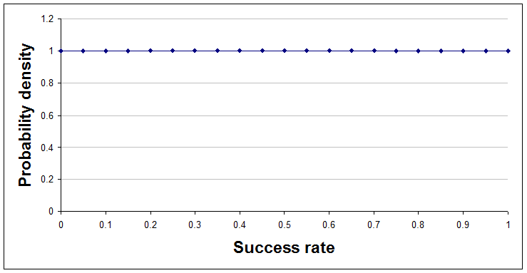
With no data so far, a=1 and b=1.
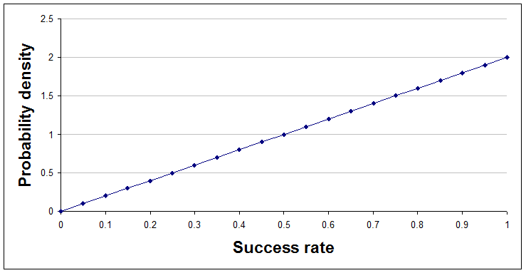
After one success and no failures, a=2 and b=1.
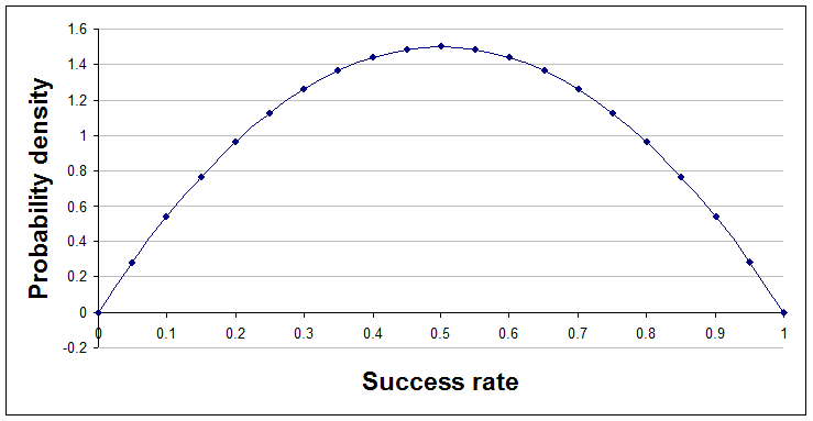
After one success and one failure, a=2 and b=2.
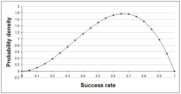
After two successes and one failure, a=3 and b=2.
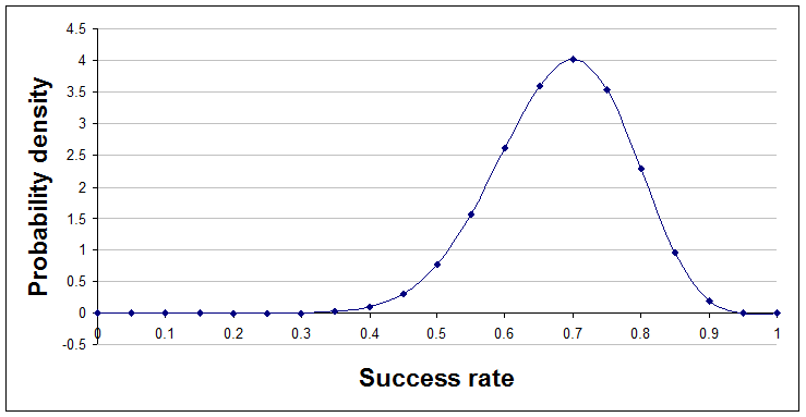
Jumping ahead a little, here's the position after 14 successes and 6 failures, a=15 and b=7.
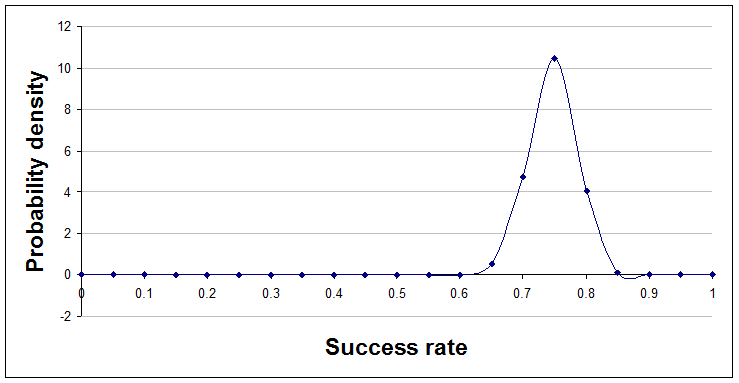
Finally, here's the position after 96 successes and 32 failures, a=97 and b=33.
A quick look at the curve, as it evolves, gives you a sense of where the truth probably lies, and further calculations or additional graphs can answer questions like "How likely is it that the rate of success is more than 70%, given the evidence we have so far?"
The technicalities explained
Here's a quick explanation of the technicalities, with plain English translation.
| Technical terms | Explanation |
|---|---|
| The curves are probability density functions on the interval from 0 to 1. | A probability density function shows how likely you think each rate is. The rate can be between 0 and 1, representing 0% to 100%. Probability density functions never go negative, but they can reach high peaks. The area under the curve is always exactly 1. |
| The curves represent beta distributions, having parameters a and b. | The beta distribution is a mathematical formula that can describe many different shapes of curve depending on the values of two numbers used within it. These numbers are called parameters and the parameters for the beta distribution are usually called a and b. |
| The beta distribution is a conjugate distribution for Bernoulli trials. | The beta distribution being a 'conjugate' distribution just means that the curve before and after sample results are processed remains a beta distribution, but with modified parameter values. It is the crucial changes to the parameter values that cause the curve to change its shape. A Bernoulli trial is just something that must have one of two values, at random. |
Doing it in Excel
Processing new results
Incredibly, working out the curves in response to new data needs nothing more than the ability to count. However, if you want to produce graphs or answer questions about the curves then you need to use Excel's BETADIST() and BETAINV() functions.
To work out the right values for the parameters a and b you just add the results from your sample to the values you had for a and b initially, like this:
new a = old a + errors found
new b = old b + ok items found
(It doesn't have to be 'errors' literally. If you were interested in how many visitors to a website go on to buy from you then you could replace 'errors' with 'conversions'. I prefer to add the interesting results to a and the others to b. Whatever you choose, make sure you are consistent.)
The very first values you use for a and b will be 1 and 1 respectively if you think all rates are equally likely. For example, if you started with the flat line representing the view that all rates are equally likely, then tested 10 items and found 2 errors, then you would update a and b to a = 3 (i.e. 1 + 2), and b = 9 (i.e. 1 + 8).
Looking at results
Watching the beta curve as it changes shape in response to new results is interesting and reassures you that you are doing the right thing.
To show the curves in a graph you need to make a table where the first column is rates, evenly spaced, between 0 and 1. The second column needs to be the value of the beta curve for that rate. You then add a scatter graph with joining lines to that and you're done.
Sadly, Excel does not provide a function to give the value of the beta curve at particular points. What it provides is BETADIST(), which gives the area under the curve from rate 0 up to a rate you specify. You can use this, with difficulty, to make a rough graph of the curve but an easier approach is to define two new functions that look like this:
Function beta_dens(r, a, b)
    beta_dens = Exp(Application.GammaLn(a + b) - Application.GammaLn(a) - Application.GammaLn(b)) _
        * r ^ (a - 1) * (1 - r) ^ (b - 1)
End Function
Once you work out how to add a 'macro' to an Excel file in your version of Excel you should be able to just copy and paste the above code into place. Once there the beta_dens() function will work in your spreadsheets like any other function, though you might not be able to find it in the function wizard and there are limits to how large a and b can be. The parameters are r (the rate expressed as a number between 0 and 1), a, and b, corresponding to the parameters of the beta curve you want to show.
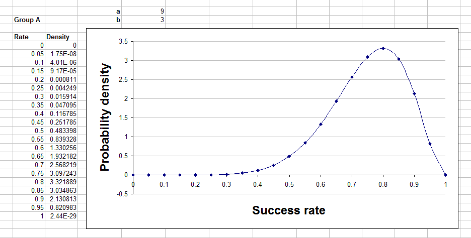
Your table and graph will look something like this:
Summarising results so far
Graphing the curve is comforting and gives you a sense of how things are developing, but to summarise the situation precisely with numbers you need Excel to do some simple calculations. Here's how to do some different types of summary number.
Comparison with a threshold
Sometimes a helpful summary of your analysis is to say how likely it is that the true rate is above (or below) a stated threshold. For example, you might say something like "I'm 91% confident that the error rate from this machine is less than 1%." or perhaps "We are 78% confident that the rate of sales conversion success will be more than 20%."
The Excel formulae for this are quite easy and use Excel's built in BETADIST() function. In the following formulae a and b are the parameters of the beta distribution you have calculated and threshold is the threshold. Obviously you need to replace these with numbers or references in your spreadsheet.
To find the probability of the truth being below the threshold use:
= BETADIST(threshold, a, b)
To find the probability of the truth being above the threshold use:
= 1 - BETADIST(threshold, a, b)
The probability of the true rate being exactly equal to the threshold, when using the beta distribution, is always zero.
A central region
For most values of a and b that you will encounter the beta distribution looks like a hill with just one peak. When it has this shape it makes sense to summarise the curve by stating a range of rates that captures most of the area under the curve. This is the fat middle of the curve, rather than the thinner tails.
To find the probability that the truth lies between a lower and an upper threshold you have chosen use:
= BETADIST(upper, a, b) - BETADIST(lower, a, b)
To find the probability that the truth lies between the 10th and 90th percentile of the curve (i.e. an area that contains 80% of the probability) use the BETAINV() function like this:
	10 percentile level = BETAINV(0.1, a, b)
	90 percentile level = BETAINV(0.9, a, b)
You could say, for example, something like "I am 80% confident that the true rate lies between 2.1% and 5.3%."
Perhaps the most attractive summary of this type is to give the range that is the narrowest one that captures a given amount of the probability. Unfortunately, this is not possible with Excel's built in functions, though you could do it with the Solver add-in.
A number to bet with
Having a distribution over all possible rates is informative and helpful. It's much better than just having a best estimate of the true rate. However, what do you do if you have to make a decision, or perhaps place a bet, given that distribution? For decision-making purposes it is generally better to hold on to the full distribution and use it in your decision model than to summarise into one number.
However, for some purposes a summary number is appropriate. For example, suppose you've tossed a bent coin a few times and then want to know the probability of throwing heads on the very next throw. What you need is the average rate of heads, with the rates weighted according to the height of the beta distribution curve. That means that rates near the high, fat part of the curve will have more influence on the average than others.
The number you need is the mean of the beta distribution, which is simply:
mean = a / (a + b)
Comparing rates
A very common requirement is to compare two or more rates. The statistical significance test for this is the Chi Square test, so the technique explained next is a direct replacement for this statistical test in this situation.
If you apply the usual beta distribution technique described above to each of the rates you are interested in then you will get parameter values for two beta distributions. Looked at on a graph they might look something like this:
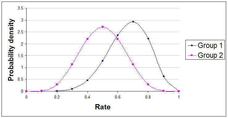
Here are examples of useful summary statements about the difference between these two curves that you might make:
"The true rate of Group 1 is 79% likely to be greater than the true rate of Group 2."
"We are 61% confident that Group 1's rate is at least 10% higher than Group 2's rate."
Unfortunately, Excel does not have a built-in function for calculating the probabilities needed for these statements, but once you know how to add new functions to your version of Excel you can paste this code in and create a new function to do it.
Function beta_diff_prob(a1, b1, a2, b2, diff, runs)
    Dim count As Long
    If a1 <= 0 Or b1 <= 0 Or a2 <= 0 Or b2 <= 0 Or runs <= 0 Or diff > 1 Or diff < -1 Then
        beta_diff_prob = "Invalid input - sorry."
    Else
        count = 0
        For i = 1 To runs
            If Application.BetaInv(Rnd(), a1, b1) > Application.BetaInv(Rnd(), a2, b2) + diff Then
                count = count + 1
            End If
        Next i
        beta_diff_prob = count / runs
    End If
End Function
In your spreadsheet you can use it as:
=beta_diff_prob(a1, b1, a2, b2, diff, runs)
The parameters need to be replaced with numbers or cell references, as follows:
a1 is the a parameter for the first beta distribution
b1 is the b parameter for the first beta distribution
a2 is the a parameter for the second beta distribution
b2 is the b parameter for the second beta distribution
diff is the difference between the two that you want to study, expressed as a number between -1 and +1. The function tests the probability that the true rate for the first curve is greater than the true rate for the second curve + the diff. If you give a diff of zero then the test is just whether the true rate of the first curve is higher than the true rate of the second curve.
runs is the number of simulations used to get an answer. The larger this number the more accurate the result, but the longer it takes to get a result. Try 100 at first to see how long it takes on your system.
If you have more than two beta distributions to compare then you can compare them in pairs and report your findings.
Generating random numbers
You might for some reason want to generate random numbers that conform to the beta distribution. (This is done in the function above, for example.) The Excel formula to generate a single such number every time the spreadsheet is recalculated is:
=BETAINV(RAND(), a, b)
As usual, a and b are the parameters of your beta distribution.
Sample sizes
With this approach to statistics there is no need to decide on your sample size in advance. You can just test items one at a time and stop the moment your results are clear enough for your purposes.
Of course it can be helpful to have some idea in advance of how many items you might need to examine. To explore this just try possible sample sizes and rates and see what the beta distributions would look like.
If you do you will soon notice that the number of items needed depends on what the results turn out to be. The common idea that you can and should decide exactly what size of sample to use in advance is wrong and causes unnecessary stress. It also leads to testing more items than you need, on average. This is due to the tendency to choose a sample size that is large enough to give you a high confidence of achieving the result you hope for. To be that confident you need a sample size that covers those situations where the sample data are unrepresentative and against your expectations.
Multiple analyses
With statistical hypothesis testing it is very easy to run into problems because of doing multiple tests. You might think that there is only a 5% chance that a 'significant' difference was just the result of a coincidence, but if you do the same test 100 times you should expect to see such differences 5 times on average. In theory, significance levels should be adjusted to account for multiple tests, though few people do this.
Happily, with Bayesian analyses there is no 'testing' of hypotheses and no attempt to reduce shades of grey to just black or white. You can do as many analyses as you like and the results of each one stand, unaltered.
Limitations
The examples of summary statements given above should really have been prefaced with the words "given the data used and the assumptions made," because we sometimes have a choice about which data to use, and because different results will arise if different assumptions are made. In this case the assumption was that items were randomly sampled. If, instead, you wanted to compare two web pages to see which best encourages people to stay on the website, you would probably compare two versions of the page for a period of time then see what the results say. This is not a random sample from the whole population of visitors that will ever visit the pages, so the assumption is not really true. This may or may not be important.
More sophisticated readers will be able to point to other ways in which assumptions might be wrong, and will also have opinions about the correct prior distribution to use. Some will favour the prior a=0.5 and b=0.5 to the uniform prior illustrated above. They might know techniques to use when there is a reason for thinking that two rates are likely to be similar, or when there is a reason to think that the rate will be one particular number. They will notice that some of my functions stop giving values for large a and b (because they involve using numbers that are either too large or too small for Excel to represent them).
Weaknesses like this are typical for the frequentist statistical tests too. Many journal papers in business and psychology (for example) contain statistical tests applied by people without a special skill in statistics and the techniques explained above are intended as a simple alternative to the more often used frequentist tests.
Finally
This recipe covers just rates for populations and events where there are only two possibilities. Similar techniques exist for a number of other situations and will be covered in future articles.
Made in England